Bank Stocks: Dividends or Patience? A Decade of Data on A-Share Core Holdings
Using a fixed sample of ten bank stocks tradable in 2015, this study traces total returns and dividend cash flows, then tests the capital, governance, and holding constraints behind a long-term core position through credit-cycle, financial-accelerator, balance-sheet-repair, FCFE, and residual-income frameworks.
长期持有银行股,最容易被看见的是分红,最容易被低估的是拿到分红之前要承受什么。本文的历史情景里,50 万元起步、按规则追加资金,最终形成了可观的股票与现金资产;但同一条路径,也曾从高点回撤近四成,历时两年多才收复旧高。因此,“银行股是 A 股长期底仓”值得认真讨论,却不能只靠高股息或国有背景来论证。我们要把总回报、资本约束、股东治理与持有纪律放进同一张研究地图,再问:什么条件下,这个命题才成立?
股票价格还多了一层预期定价:它可以在财报改善前反映投资者对修复的期待,也可以在利润仍增长时,因为风险溢价上升而下跌。因此,经济活动的底、信用损失的高点、普通股利润的底和股价的底,不应被当作一个时点。看到经济指标回升才买入,并不自动是低价;看到股价先反弹,也不证明资产质量已经恢复。本文讨论的是这些错位的可能机制,没有估计它们在 A 股中的固定领先月数。
BIS 2018 年关于金融周期与衰退风险的研究,使用了 16 个发达经济体 1985—2017 年的季度数据。这个样本边界很重要:它支持认真研究金融变量与衰退的关系,却不能直接给出中国银行股的买入年份、目标市净率或加仓阈值。来源:《The financial cycle and recession risk》。周期理论的用途,是提醒我们不要用一个短时钟解释全部长期风险。
The most visible reward from holding bank shares for years is the dividend. What is easiest to underestimate is what an investor must endure before receiving it. In this historical scenario, an initial RMB 500,000 account with rule-based additions eventually held substantial stock and cash. The same path also fell nearly 40 percent from its high and took more than two years to recover. The claim that banks can form a long-term core allocation in China’s A-share market deserves serious study, but a high yield or state ownership cannot establish it. Total return, capital constraints, shareholder governance, and holding discipline belong on the same research map.
Define the core-holding claim before judging it
Here, a “core holding” is neither a trading basket for predicting short-term moves nor a concentrated industry bet. It is an equity position intended for low-turnover, long-duration ownership while remaining subject to continuing risk review. The case for putting banks in that role is that they remain central to household saving, business finance, and payment clearing; mature banks regularly disclose profits, capital, and distribution policy; and their ownership and regulatory structures make risks open to inspection. None of this means the state protects every common shareholder from loss.
At the end of the fourth quarter of 2025, China’s banking financial institutions reported RMB 480 trillion in assets. Commercial banks reported a 1.50 percent non-performing loan ratio, 205.21 percent provision coverage, and a 15.46 percent capital adequacy ratio, while net interest margin had fallen to 1.42 percent. The sound reading is that capital buffers remained and margin pressure was real. The asset total and the four ratios do not use identical reporting populations, and industry averages cannot substitute for analysis of one bank. See the National Financial Regulatory Administration indicators republished by the China Banking Association.
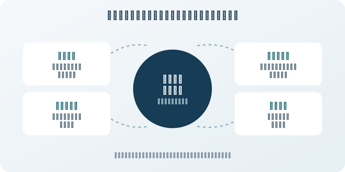
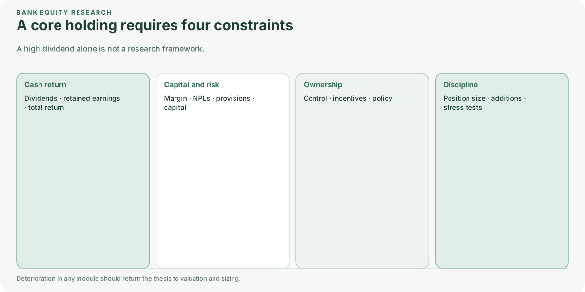
Diagram | Bank research is not a high-yield screen. It is four mutually constraining modules.
The ten securities below are therefore a fixed research sample that was tradable in 2015, not a current top-ten list or a recommendation: ICBC (601398), China Construction Bank (601939), Agricultural Bank of China (601288), Bank of China (601988), Bank of Communications (601328), China Merchants Bank (600036), Industrial Bank (601166), Ping An Bank (000001), Bank of Ningbo (002142), and Bank of Nanjing (601009). The set includes large state banks, joint-stock banks, and city commercial banks so that different funding structures, regional exposures, and governance are not compressed into one “bank” label.
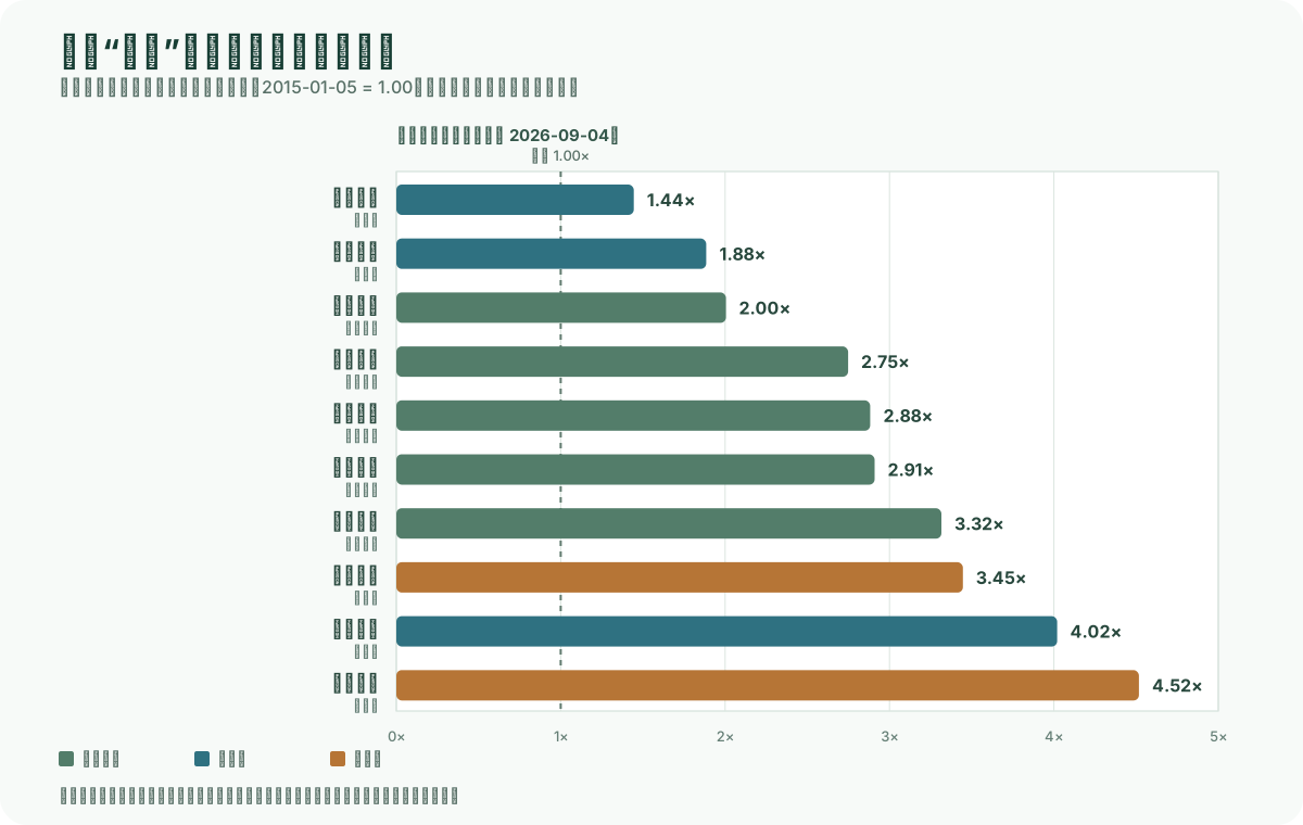
The results require that caution. From January 5, 2015 to September 4, 2026, the ten securities’ pretax dividend-reinvestment total-return indices ended between 1.44 and 4.52, a ratio of roughly 3.13 between the highest and lowest. Those indices reinvest dividends at the ex-date close. The portfolio account later in the article retains dividends as cash, so the two measures must not be mixed. Industry diversification reduces dependence on one bank; it does not make earnings quality, capital consumption, or governance identical. An industry average conceals the selection risk an investor actually carries.
Figure 1 | Dispersion in realized history. Each stock uses a pretax dividend-reinvestment index including stock distributions and excluding trading costs. It is not the cash-dividend account below. “Banks” is a starting point for research, not a substitute for company analysis.
A dividend is cash flow, not total return
A long-term shareholder receives more than a static yield. Return combines cash paid out, retained capital that continues to produce profit inside the bank, and the market’s repricing of future asset quality, rates, and capital constraints. The first two are traceable in reports and distribution plans; the third can produce large price movements. Yield alone mixes cheap valuation, low growth, rising risk, and a one-time high payout.
Net interest margin illustrates the tension. The People’s Bank of China’s first-quarter 2025 monetary-policy report discussed rates, credit delivery, and financial-institution operations within one macro framework. Investors should treat margin, funding cost, loan repricing, and credit cost as linked variables rather than extrapolating a quarter’s profit forever. The original report is available for review.
For a core position, a more useful sequence is:
Begin with capital ratios, provisions, new non-performing formation, and write-offs to judge whether dividends can survive loss absorption.
Examine margin, non-interest income, and cost-to-income ratio for the durability of profit.
Compare payout, cash flow, and capital-raising plans to separate distributable capacity from cash already distributed.
Only then place price-to-book, dividend yield, or a dividend model inside a comparison of risk premia.
The IMF’s 2025 Financial System Stability Assessment for China similarly put the property adjustment, local-government financing vehicles, and macro stress tests in the risk background. Low valuation is not an automatic margin of safety; correlations among risky assets tend to rise under stress. See the IMF assessment summary.
A testable approximation is more useful than “high yield”: shareholder total return ≈ cash dividend yield + growth in book value per share + change in price-to-book. Return on equity, payout, credit cost, and capital constraints jointly shape the first two terms. Expectations and required returns shape the last. This is not a precise valuation equation, but it avoids two common errors: assuming that a falling price-to-book must reverse because the stock is cheap, or that profit growth can all be paid to shareholders.
The falsifier becomes clearer. If a bank’s ROE is falling, risk-weighted asset growth still consumes substantial capital, and investors demand a higher cost of equity, distributable capacity and valuation can weaken even before the quoted yield falls. Conversely, steadily improving profit, buffers, and book value per share need not be refuted by a temporarily flat price. The object to track is continued value creation per share, not merely a return to the purchase price.
Credit, balance sheets, and capital run on different clocks
“Hold for the long run and pass through the cycle” is easier to say than to test. Banks do not only bear a cycle; credit decisions, collateral values, and capital constraints can amplify or damp it. A core-holding thesis therefore requires more than a forecast of economic recovery. Who repays debts created during the previous expansion? Who absorbs losses after collateral falls? After the losses are handled, how much profit can each common share still produce?
1. Separate four clocks instead of treating the cycle as a calendar
The BIS distinguished conventional business cycles from financial cycles in its 2014 Annual Report. The former center on output and activity; the latter on the mutual reinforcement of credit, property prices, and financing constraints. In the historical samples it discussed, ordinary business cycles often lasted one to eight years and financial cycles roughly fifteen to twenty. These are empirical features of particular samples and methods, not a law that fixes the bottom of China’s economy or A shares at regular intervals. Source: BIS 2014 Annual Report, Chapter IV.
For bank research, record four clocks separately. This is an analytical framework, not four estimated Chinese cycle series. They may overlap or diverge and can be changed by institutions and policy.
Old losses and capital repair may continue after the economy stabilizes; dividends need not turn with activity.
Share prices add a clock of expectations. They may anticipate repair before accounts improve or fall while profit grows if the risk premium rises. The bottom in activity, peak credit losses, trough in common-equity profit, and low in share prices should not be treated as one date. Buying after an economic indicator improves does not guarantee a low price; an early rally does not establish repaired asset quality. This article describes mechanisms of divergence and does not estimate a fixed lead for A shares.
A 2018 BIS study of financial cycles and recession risk used quarterly data for 16 advanced economies from 1985 through 2017. That boundary matters. It supports studying financial variables as recession signals, but it cannot provide a Chinese bank purchase year, target price-to-book ratio, or averaging threshold. See “The financial cycle and recession risk”. Cycle theory is useful because it stops one short clock from explaining every long-run risk.
2. Minsky: risk may accumulate when conditions look most stable
Hyman Minsky’s 1992 paper divided financing into hedge finance, where cash flow covers interest and principal; speculative finance, where interest can be paid but principal requires refinancing; and Ponzi finance, where operating cash flow cannot cover interest and new borrowing or asset sales maintain the position. “Ponzi” here is a theoretical cash-flow category, not an accusation of fraud; “hedge” does not refer to a hedge fund. Source: Minsky’s paper and the Levy Institute summary.
For bank analysis, the point is not to label every borrower. It is to identify the source of repayment. Does a loan rely on operating income, on refinancing at maturity, or on continuously rising collateral? All three can service interest in good times but withstand weaker cash flow and tighter finance differently.
Minsky’s warning is that a long expansion can change risk appetite and financial structure; apparent stability need not mean a growing margin of safety. The relevant bank-research question is whether a low NPL ratio reflects stronger borrower cash flow, a denominator enlarged by loan growth, renewed loans delaying recognition, or write-offs removing old balances. These are hypotheses to check, not grounds to accuse a bank of concealment. A stable NPL ratio is not a reason to stop checking special-mention loans, overdue migration, and cash collection.
3. The financial accelerator: asset prices can feed back into credit
Bernanke, Gertler, and Gilchrist’s financial-accelerator framework explains how credit-market friction amplifies and transmits macro shocks rather than treating finance as a passive conduit. Source: NBER Working Paper 6455, 1998. The implication for bank holdings is that pressure can come not only from fewer loans but also from feedback among thinner borrower net worth, tighter financing conditions, and higher credit costs.
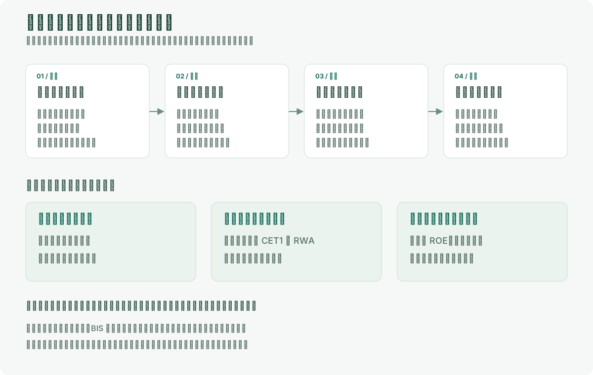
A typical collateral loop is easy to describe. Credit expansion supports asset transactions; rising assets improve collateral and financing access; more finance supports further expansion. When cash flow or asset prices weaken, the feedback can reverse. The following diagram is a mechanism, not attribution for every crisis or a measured path for China. Its central reminder is that a bank holds a loan contract backed by borrower cash flows and assets that move with the economy.
Mechanism | The cycle reaches common equity through borrowers, credit losses, and capital. This original synthesis follows the cited financial-cycle and accelerator research; it is neither dated to specific years nor a measured or inevitable sequence.
The mechanism also qualifies the phrase “defensive bank stocks.” Stable funding and mature earnings do not prevent losses from clustering under stress. Diversifying among ten banks can reduce one company’s governance or execution risk without diversifying a common change in property collateral, regional industry stress, or weak credit demand. In the historical account below, 16 additions clustered in January 2016. That is a feature of the account rules, not evidence of an identified macro turning point.
4. Balance-sheet recession: why cheap money may not create borrowing
Richard Koo’s 2011 paper used Japan after its asset bubble to describe a mechanism different from ordinary demand fluctuation. When asset values fall but debt remains, firms and households may prioritize debt reduction and balance-sheet repair over new borrowing and investment. Low rates and abundant liquidity may then fail to restore private credit demand quickly. Source: “The world in balance sheet recession: causes, cure, and politics”, especially the opening mechanism and Japanese case.
Two effects should be separated in bank analysis. A lower financing burden may reduce borrower defaults, while active deleveraging and deferred investment weaken demand for good loans. Both can occur. “Rate cuts help the real economy” does not translate directly into “bank profits rise.” Bank returns also depend on asset yield, deposit repricing, credit losses, and whether new assets cover the cost of capital.
This is a conditional explanation, not a label for China as a whole. Testing it in an industry or region requires borrower net financing, debt service, investment, and cash flow. A news item or a falling share price is insufficient. Japan’s experience does not establish that China must repeat the same duration.
5. China: financial stability and shareholder profitability need separate tests
The IMF’s April 4, 2025 Financial System Stability Assessment for China is directly relevant. It credited regulatory reforms and the capital and liquidity buffers of large banks while also pointing to property adjustment, local-government financing vehicles, the effect of accommodative monetary conditions on organic profitability, and the greater vulnerability of some smaller banks. It supports neither simple optimism nor pessimism. Stability and profitability must be verified separately. See the IMF summary. It describes that assessment, not a live risk rating for September 2026.
Debt extension can relieve a borrower’s current principal burden without raising the project’s future income. A capital injection can increase a bank’s loss-absorbing and lending capacity, while the new share count, issue price, and later return on capital determine whether existing shareholders benefit. The Ministry of Finance, Central Huijin, and local-state actions described later belong in two separate chains: one tests credit and institutional stability; the other tests earnings, book value, and distributions per common share. Policy support does not prove the core-holding case if the second chain is omitted.
The Basel Committee’s 2010 countercyclical capital-buffer guidance makes the same distinction. Its purpose is to build protection when excess credit growth raises systemic risk and release it under stress to reduce the effect of capital constraints on credit supply. Source: BCBS guidance. This explains an international framework, not a claim that China had made a particular release. Applicable domestic requirements and bank-level rules must be checked. Protecting financial intermediation does not guarantee a common-equity return at every purchase price.
6. Put the cycle into valuation without making the best year perpetual
The FCFE, dividend, and residual-income models below need more than the latest ROE. They need assumptions that pass through loss recognition and capital repair. A practical approach separates pre-provision operating capacity from credit cost and asks whether favorable years relied on unusually low losses, rising assets, or rapid loan expansion. A ten-year simple average is not automatically cycle-neutral if the sample never includes concentrated loss recognition.
Stable ROE deserves special care. A high ROE under low credit costs should not enter a terminal value unchanged; weak profit under stress need not mean permanent impairment. The question is whether losses are a one-time clearing of a stock problem or whether the business persistently fails to cover credit and capital costs. This worksheet organizes scenarios and does not classify the ten banks today.
Analytical scenario
Variables that should move together
Falsifier that cannot be skipped
Expansion
Faster loan/RWA growth, possibly low current credit cost, greater retained-capital need
Does high ROE depend on excess expansion or refinancing borrowers? Can high growth coexist with high payout?
Loss recognition
Higher credit cost, lower profit, possible capital deductions or risk-weight changes
Is the dividend consuming buffers? Will a capital gap require new common shares?
Balance-sheet repair
Loss recognition and disposal, funding-cost adjustment, gradual borrower cash-flow recovery
Is cash collection improving, or have repayment and recognition merely been delayed? What capital and time does repair consume?
Normalization
Sustainable ROE, normal credit cost, supportable RWA growth and payout
Does the model restore peak profitability too soon? Are growth and retained capital consistent?
Nor does “the cycle returns” mean price-to-book must revisit its old high. A weaker funding advantage, competition that lowers normalized margin, or permanently higher capital requirements can reduce normal ROE. Economic activity may revert without restoring the old profit center. A cycle can support the holding case only if the mechanism of common-equity value creation remains intact.
7. When averaging down, ask whether price or the premise became cheaper
Cycle research does not replace trading rules, but it reveals their blind spots. The 20 and 35 percent drawdown thresholds below use price and dividend indices only. They observe neither borrower repayment, bank buffers, dilution, nor macro cycles. They form a mechanical historical scenario, not a validated “buy the cycle bottom” strategy. Nothing in this section changes the backtest or gives its thresholds retroactive theoretical authority.
A better next step puts current price drawdown alongside credit fragility, bank buffers, and value-per-share changes. BIS research on early-warning indicators for banking crises examined credit-to-GDP gaps and debt-service ratios. The first measures credit’s deviation from trend; the second principal and interest burden relative to income. These are systemic-risk tools, not stock-return forecasts or ready-made Chinese trading signals. Source: Drehmann and Juselius, BIS Working Paper 421, 2013.
Three review questions follow. Does the borrower still have a source of repayment? Can the bank maintain its capital requirement after recognizing reasonable losses? Under the current share count, can common dividends and normalized ROE still support the valuation? The aim is not to call the exact bottom but to distinguish a lower price on an intact foundation from a lower price accompanied by weaker value.
Any future macro backtest must preserve the data actually published at each date and its release lag, including revisions and endpoint problems in trend estimates. Today’s complete history cannot be used to pretend that an investor saw the cycle bottom at the time. For holding discipline, cycle theory is most useful when it encourages cash preparation for long repairs instead of using “already down a lot” to exhaust every addition too early.
A 2015–2026 scenario: RMB 500,000 plus up to RMB 500,000
This is neither a forecast nor a directly reusable recommendation. Fixed parameters set today are applied to history. The narrow question is what happened when ten sample stocks began at equal weights in early 2015 and received mechanical additions after large drawdowns, combining prices with pretax cash dividends. It does not imply that an investor in 2015 had already selected these parameters or companies for these reasons.
The thresholds were triggered in 2016 and 2022, so the rule used only RMB 425,000 of the RMB 500,000 additional capacity. “Up to” does not mean the full amount must be deployed.
Scenario
External contributions
Value on 2026-09-04
Pretax dividend cash within value
Cumulative return on contributed capital
Money-weighted annual return
Maximum drawdown (time-weighted)
RMB 500,000 initially, no additions
RMB 500,000
RMB 1.202m
RMB 313,000
140.5%
7.8%
-36.9%
RMB 500,000 initially, rule-based additions
RMB 925,000
RMB 2.282m
RMB 572,000
146.7%
8.5%
-36.9%
RMB 1m invested once in early 2015
RMB 1m
RMB 2.415m
RMB 629,000
141.5%
7.9%
-37.1%
Separate three return measures
Cumulative return is ending value divided by actual cumulative contributions minus one. It ignores contribution dates and cannot be annualized by dividing by years. Money-weighted annual return (XIRR) uses each contribution date and ending value to answer what the invested money earned along that funding path. Time-weighted return removes the effect of external cash flows day by day to describe the account’s internal asset growth. The model treats contributions as arriving at the start of a trading day, marks stocks at the close, and pays no interest on cash.
The three time-weighted annual returns were about 7.65, 7.65, and 7.69 percent. The 8.5 percent XIRR for rule-based additions minus the 7.8 percent XIRR without additions is therefore not repeatable stock-selection or timing alpha. Contribution timing, holdings, and cash all affect it. The one-time RMB 1 million scenario ended higher partly because more money entered earlier.
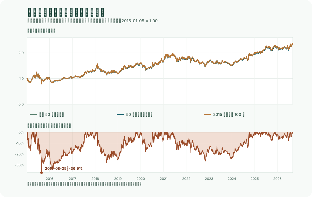
Figure 2 | The curves ask whether the path was bearable, not whether the endpoint is attractive. Both use complete daily data. The upper chart removes external cash-flow effects; the lower shows the rule account’s realized maximum drawdown.
The -36.9 percent path is the number not to overlook. The account reached a high on June 8, 2015, hit maximum drawdown on August 25, and did not exceed the old high until August 2, 2017—786 calendar days later. Ending with RMB 2.282 million did not make the experience easy. An investor unable to accept a fall near 40 percent, or unwilling to continue the rule afterward, could not realize the terminal figure. Additions raised the money-weighted return in this sample but did not remove drawdown or prove that the next stress period will follow the same sequence.
The “diversified” addition rule was not diversified in stress. All ten first additions at a 20 percent drawdown executed on January 12, 2016. Of seven second additions at 35 percent, six occurred in January 2016 and one for China Merchants Bank on May 10, 2022. Sixteen of seventeen additions clustered in one month. The rule was still in its 250-day warm-up during the 2015 maximum drawdown, so this does not establish that additions generally fail to reduce drawdown. It does establish that ten banks did not create seventeen independent opportunities. Holding ten banks does not create ten independent sources of risk under common credit, liquidity, and rate stress.
Figure 3 | Historical cash-dividend ledger. The 2026 bar is a partial period through September 4. Amounts are pretax, not reinvested, and recognized by the model on ex-dates rather than actual bank-account payment dates.
Figure 3 does not show dividend capacity compounding at that rate every year. Concentrated additions in 2016 increased the share count; stock distributions and later additions changed it again. Company dividend growth requires decomposing total cash into shares held times dividend per share.
The ending account reconciles as follows: RMB 1.6933 million in stock + RMB 572,100 in pretax dividend cash + RMB 16,700 left after whole-lot purchases = RMB 2.2821 million. Total commission of RMB 272.41 was deducted in purchase costs. The unused RMB 75,000 addition budget never entered the securities account and is not in its cash or value. If treated as household reserve cash earning zero, the full RMB 1 million budget ended at RMB 2.3571 million, a cumulative 135.71 percent. That household-budget denominator must not be mixed with the RMB 925,000 actually contributed in the table.
What did each bank contribute?
The ledger below is from the rule-based scenario. Amounts are RMB 10,000 and rounded to two decimals. “Budget” includes unspent remainder after purchases; “purchase cost” includes commission. Dividend cash is already inside account cash and must not be added again to ending value.
Bank
Budget
Purchase cost
Ending stock value
Cumulative pretax dividends
Additions
ICBC
7.50
7.47
12.85
5.01
1
China Construction Bank
10.00
9.85
18.67
6.58
2
Agricultural Bank of China
7.50
7.45
14.76
4.92
1
Bank of China
10.00
9.95
16.75
5.96
2
Bank of Communications
10.00
9.91
11.65
5.80
2
China Merchants Bank
10.00
9.53
21.26
7.47
2
Industrial Bank
7.50
7.26
8.02
4.35
1
Ping An Bank
10.00
9.85
11.73
3.41
2
Bank of Ningbo
10.00
9.78
33.73
6.12
2
Bank of Nanjing
10.00
9.77
19.93
7.61
2
Source: local calculation output rule_additions_per_bank.csv. This is not a return ranking: contribution dates and amounts differ, and the portfolio is not rebalanced. Initial equal weights do not remain equal. Bank of Ningbo ended at about 19.9 percent of stock value, nearly twice its initial 10 percent. Whether to restore target weights is a separate strategy question.
The script, orders, daily net asset value, individual dividends, and de-duplicated corporate-action records are stored with the repository under research/experiments/a_share_bank_core_holdings_v1/ and can be recalculated on the same basis. “Dividend contribution” means pretax cash not reinvested; total return includes that cash alongside closing market value.
This study has no CSI 300, bank index, or dynamic investable-universe control. It cannot answer whether the ten-bank portfolio beat an index. It answers only what happened to a fixed sample under a fixed corporate-action treatment and addition rule. A return chart without a control cannot become a relative-performance claim. Adding the missing comparison is a falsification design for later work, not a detail to omit from the prose.
Three more boundaries remain. Cash is recognized on ex-dates even though the real spendable date may be later. Stock distributions are rounded to holdings, without modeling every clearing remainder, rights subscription, or corporate action. The calculation uses local caches and has not independently cross-audited every quote and action against issuer notices. “An account model using real historical inputs” is more accurate than “brokerage-account performance.” The common cache cutoff is September 4, 2026, not the full month or publication date, and policies discussed after September 7 are not inserted retrospectively into the test.
A bank is not valued like an ordinary company’s free cash flow
“Use a DCF” should not mean subtracting capital expenditure from a bank’s operating cash flow and calling the remainder free cash flow. Deposits, loans, reserves, and regulatory capital are the operating cycle itself. Treating them like a manufacturer’s working capital often produces a misleading number.
A better translation of free-cash-flow thinking is capacity distributable to common shareholders, cross-checked through at least three frameworks:
Framework
Core question
Inputs that matter most for a bank
FCFE
After growth and regulatory capital, how much cash can common equity receive?
Net income, RWA growth, target capital ratio, capital issuance
Dividend discount model
What is the present value of paid and sustainable dividends?
Long-run payout, earnings growth, cost of equity, capital constraint on distributions
Residual income
Can future ROE remain above the cost of equity?
Opening book value, ROE, cost of equity, retention rate
One auditable approximation is sustainable dividend ≈ net income − retained capital needed to maintain the target capital ratio. In residual income, value begins with opening book value + the present value of future (ROE − cost of equity) × opening book value. Neither produces one automatic price target. Both require internally consistent assumptions about ROE, credit cost, capital, and growth.
A full equity DCF discounts each period’s distributable cash: common-equity value = Σ FCFE_t / (1 + Ke)^t + terminal value / (1 + Ke)^N, where Ke is the cost of common equity. Under stable growth, terminal value = FCFE_(N+1) / (Ke − g). This is not a WACC discount of free cash flow to the firm, and proceeds from issuing shares are not sustainable cash produced for existing holders. As growth approaches the cost of equity, terminal value becomes extremely sensitive; a model should disclose the terminal share of total value instead of showing only its final price.
In practice, each bank needs low, central, and high cases that connect margin narrowing or stabilization, credit-cost increases or declines, faster or slower RWA growth, and payout constrained by capital. If the high valuation requires both permanently high ROE over the cost of equity and no future capital need, it is fragile. Here, DCF exposes assumptions; it does not certify a volatile market price.
Translate “free cash flow” into a capital constraint
The common error in bank FCFE is to treat cash from operations as distributable. Deposit inflows, new lending, and interbank positions are ordinary banking activity, not inventory adjustments to remove from free cash flow. A first approximation closer to the common-equity constraint is:
Retained capital required to maintain target CET1
≈ target CET1 ratio × increase in risk-weighted assets (RWA)

Sustainable capacity for common dividends
≈ profit attributable to common equity − required retained capital
  − new regulatory deductions / buffer requirements
  (then account for dilution from external common-equity issuance)
This is not a regulatory reporting formula. Actual CET1 also reflects other comprehensive income, deferred tax, capital instruments, and deductions. RWA can change because of weights rather than loan growth. The approximation nevertheless forces a neglected question: How much common equity must be locked up for one additional unit of RWA? A model that assumes high growth, high payout, and no financing must identify the source of the capital.
Profit must also match the claim. Distributions owed to preferred shares, perpetual capital securities, and other equity holders should be deducted from profit attributable to the parent before discussing common dividends. If the target capital ratio rises, existing RWA also requires more capital. External issuance replenishes capital but is not free cash flow created by existing holders.
In a stable-growth DDM or residual-income check funded by retained profit, g ≈ ROE × retention rate, and P/B ≈ (ROE − g) / (cost of equity − g). ROE must use opening common book value, cost of equity must exceed growth, and the simplified relation assumes no new share issue and continuity between earnings and book value. It is a consistency check rather than a quote. A low P/B can mean low sustainable ROE or a high required return; those interpretations have very different portfolio implications.
A worked example: high growth need not mean high payout
Every number in this example is illustrative and refers to no bank’s actual accounts or price target. Assume RMB 10 billion of common profit, opening RWA of RMB 1 trillion, and a 10 percent target CET1 ratio that is exactly met. Five percent RWA growth adds RMB 50 billion of RWA and needs roughly RMB 5 billion of common capital, leaving simplified distribution capacity of RMB 5 billion. At eight percent growth, RMB 8 billion must be retained, leaving RMB 2 billion. If the target ratio also rises from 10 to 11 percent, the five percent growth case raises required capital from RMB 100 billion to RMB 115.5 billion. Profit of RMB 10 billion cannot cover the RMB 15.5 billion increase, much less be fully paid out.
Now use a stable-growth cross-check with long-run growth fixed at three percent. The theoretical P/B values below are model scenarios, not forecasts.
Sustainable ROE
Cost of equity 9%
Cost of equity 10%
Cost of equity 11%
8%
0.83x
0.71x
0.63x
10%
1.17x
1.00x
0.88x
12%
1.50x
1.29x
1.13x
At 10 percent ROE and three percent growth, retention is 30 percent and payout 70 percent. With a 10 percent cost of equity, theoretical P/B is one. If ROE falls to eight percent and cost of equity rises to 11 percent, theoretical P/B is about 0.63 despite positive growth. A price below book may be an opportunity or a reasonable price for weak capital returns. Profit and capital assumptions must come first.
Ask four consecutive questions of a bank DCF. Does projected profit deduct sufficient credit cost? Is RWA growth consistent with the CET1 target? Do dividends and external financing coexist without double counting? If ROE exceeded the cost of equity only in one or two favorable years, why should residual income persist? A model that survives those questions is worth comparing with market price.
Shareholders, governance, and policy belong in the research file
A bank cannot be read from the income statement alone. Control over capital raising, board appointments, and risk appetite affects common equity on both the upside and downside. As examples from 2025 annual reports, China Construction Bank and Bank of China had state-ownership structures centered on Central Huijin and the Ministry of Finance; China Merchants Bank’s largest shareholder was China Merchants Steam Navigation; Industrial Bank had major holdings from the Fujian finance department and a provincial financial-investment platform. Percentages change with reporting periods and transactions, so they should be checked in each “major shareholders” table: China Construction Bank, Bank of China summary, China Merchants Bank, and Industrial Bank reports.
The table is a control and capital-constraint worksheet, not a reduction of top shareholders to background labels. It classifies relationships to verify in 2025 reports and related disclosures without presenting trading-day-sensitive percentages. Percentages, pledges, aggregation of connected parties, and board-nomination rights require line-by-line checking against company reports and articles.
Sample
Ownership or control relationship to identify
Common-equity question
ICBC, CCB, ABC, BOC
State ownership centered on Central Huijin, the Ministry of Finance, and other state-capital holders
How do stability goals, capital support, and policy lending affect ROE, dividends, and capital per share?
Bank of Communications
State shareholders including the Ministry of Finance alongside a strategic financial investor
Does a multi-shareholder structure alter capital raising, governance, and transmission of cross-border risk?
China Merchants Bank
Important direct and indirect holdings in the China Merchants group; the annual report also says it has no controlling shareholder or actual controller
Do not confuse influence of the largest shareholder with legal control; how do the board, related transactions, and capital plans operate?
Industrial Bank
Fujian’s finance department and wholly owned Fujian Financial Investment together form the disclosed large holding and appoint directors
Does a local fiscal/financial platform bring both a capital and governance role and regional policy exposure?
Ping An Bank
Controlled within the Ping An insurance group
Are group resources, retail strategy, and capital plans aligned with return per share for minorities?
Bank of Ningbo
Local Ningbo state capital and overseas strategic investors among a diverse shareholder base
Are local exposure, the strategic investor’s role, and equity stability sustainable?
Bank of Nanjing
Local state capital, financial institutions, and industrial capital in a diverse structure
How do ownership changes, local related risk, and outside capital alter governance and dilution?
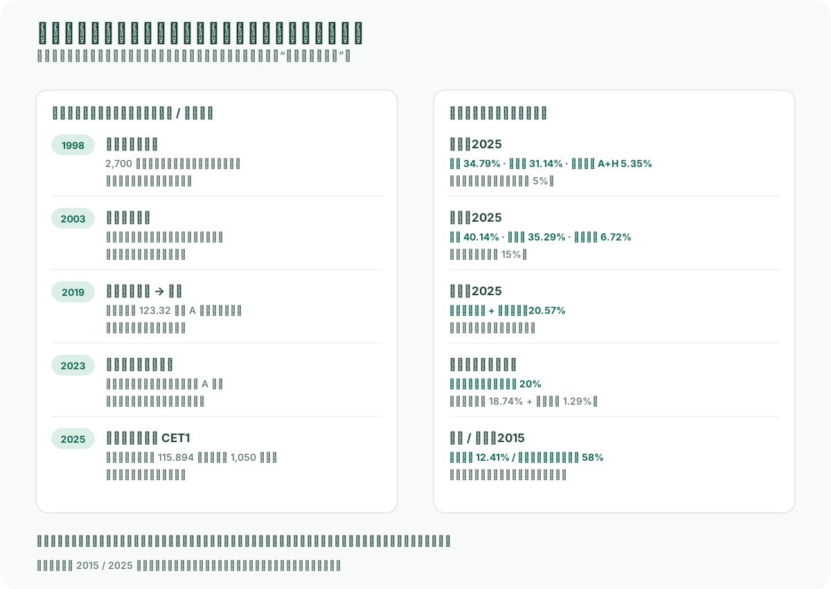
The purpose is not to score shareholders. It is to separate three chains. The ownership chain determines who has influence at critical moments. The capital chain determines who supplies capital after losses and whether existing value per share is diluted. The risk chain maps exposure to local government, property, interbank markets, or group customers. They may overlap or diverge. Industrial Bank’s public major-shareholder assessment, for example, reported a combined 20.57 percent holding by the Fujian Department of Finance and Fujian Financial Investment at year-end 2025, with appointed directors. That is a verifiable ownership and governance fact, not a dividend or price forecast. See the original disclosure.
The stronger question is which national or local body acquired, transferred, or increased which right, on what date, through which legal and capital instrument. Ministry of Finance special bonds, Central Huijin’s investor holdings, transfers of state capital to the social-security fund, and local state-platform shares are not one form of support. An insurer’s control of Ping An Bank is another corporate relationship and does not become government ownership because it sits in a financial group.
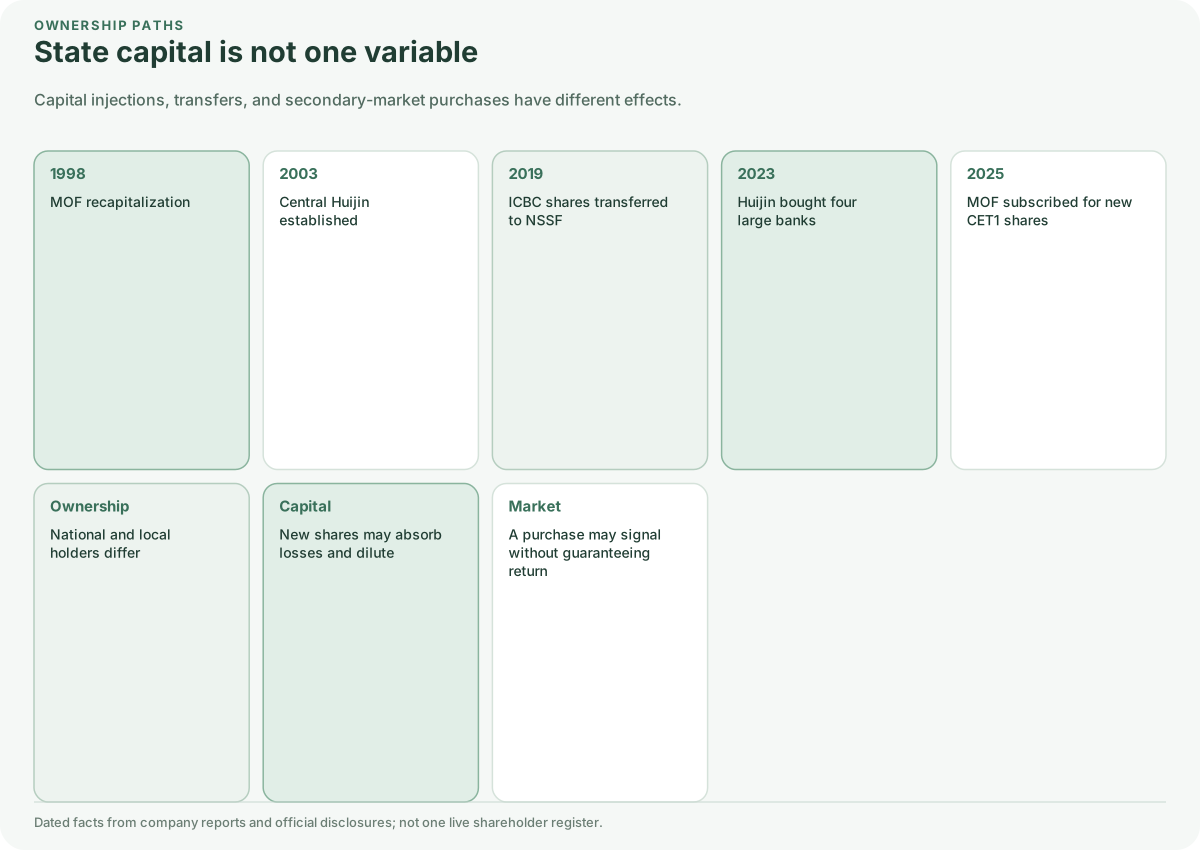
Figure 4 | Paths of national and local state capital. This is not a complete shareholder register on one trading day. It juxtaposes different dates, actors, and actions so that capital injections, state-share transfers, and secondary-market purchases are not treated as one event.
The figures in the diagram return to primary disclosures. ICBC’s 2025 major-shareholder assessment reported combined A- and H-share holdings of 34.79 percent for Central Huijin, 31.14 percent for the Ministry of Finance, and 5.35 percent for the National Council for Social Security Fund. Agricultural Bank of China reported 40.14, 35.29, and 6.72 percent respectively. These numbers do not show a guarantee for common equity. They show why research on per-share capital, rights, and state-capital changes must state whether multiple holders are combined. See the ICBC assessment and ABC assessment.
The historical path cannot be reduced to Central Huijin. ICBC’s 2024 annual-report summary records a 2019 transfer of 12,331,645,186 A shares from the Ministry of Finance to the state-capital transfer account of the social-security fund. That changed which state body held the capital and the applicable lock-up; it was neither a company buyback nor newly earned profit. Central Huijin’s 2023 purchases of A shares in four large state banks were secondary-market actions by a controlling shareholder. In 2025, by contrast, the Ministry of Finance subscribed in cash to private placements that replenished CET1. CCB issued 11,589,403,973 A shares and raised RMB 105 billion; Bank of China announced a Ministry of Finance subscription cap of RMB 165 billion and later completed the issue. Sources: ICBC 2024 summary, 2023 Huijin announcement, CCB 2025 report, and Bank of China completion notice.
Local and group paths change too. Industrial Bank’s 2025 material shows the combined 20.57 percent Fujian holding and appointed directors. Bank of Ningbo’s company profile says Ningbo Development Investment and parties acting in concert represent roughly 20 percent held for the government, but the profile does not date that snapshot and cannot serve as a live register. Bank of Nanjing’s 2015 report listed BNP Paribas at 14.87 percent and Nanjing Zijin Investment at 12.41 percent, illustrating an overseas financial institution alongside local state capital. Ping An Bank’s 2015 report gives a dated control history: China Ping An and Ping An Life held 52.38 percent after the 2011 restructuring, 59 percent after a 2013 placement, and 58 percent after the May 2015 placement. A 2011 historical number inside a 2015 report is not a 2015 year-end holding. Sources: Industrial Bank, Bank of Ningbo profile, Bank of Nanjing 2015 report, and Ping An Bank control history.
For common-equity research, put each state-capital action in one of three columns. Did it change the bank’s capital, rights among shareholders, or secondary-market holdings? Only the first directly raises loss-absorbing resources. The second may affect control and dilution per share. The third mainly changes market signaling. All can matter; none guarantees a common-equity return.
The policy timeline belongs beside the valuation model:
Period
Public action
Implication for common equity
1998–1999
Special government bonds recapitalized wholly state-owned commercial banks; four asset-management companies received non-performing assets
Systemic repair changes capital and balance sheets, so historical profit cannot be extrapolated alone. 1998 document; 1999 document.
2003–2005
Central Huijin was established and injected capital alongside joint-stock reform and listings
The state investor, corporate governance, and market listing are separate layers; trace the capital source, board mechanism, and value per share. Official reform review.
2019
Regulators took over Baoshang Bank
Liquidity, governance, and resolution at one institution cannot be replaced with an assumption that every bank is too big to fail. State Council report.
2023
Central Huijin increased holdings in four large state banks
A controlling-shareholder action may influence expectations but is not an unconditional endorsement of every bank valuation. Xinhua announcement.
2025
The Ministry of Finance issued the first special bonds supporting CET1 replenishment at large state banks
Capital constraints and macro policy directly affect dividends, growth, and dilution and belong in the scenario inputs. Ministry explanation.
2026-09-07
The Ministry announced an upcoming RMB 300 billion special-bond issue supporting CET1 at eight central financial enterprises including ICBC and ABC
RMB 300 billion is the total for eight institutions, not an amount for each bank or proof of completed injection. Bank-level issues, subscriptions, and receipt of capital still require verification. The notice came after the backtest cutoff. Ministry notice.
State ownership is therefore part of governance and policy transmission, not an automatic valuation factor. It may reduce some tail risks while bringing capital allocation, policy concessions, and governance aims that do not perfectly align with short-run common-equity returns. System stability, protection of depositors and creditors, and common-shareholder returns are three different things.
Long holding periods test mental accounting
Bank holdings invite two opposite errors. One treats quarterly dividends or a low P/B as permission to believe the stock cannot fall. The other discards the research framework after a worsening macro narrative and a deep drawdown. One ignores risk; the other forgets why the investor accepted equity risk in the first place.
Useful discipline is not forced optimism. Before buying, write down testable commitments. How much drawdown can I tolerate? Which deterioration pauses additions? How would a dividend cut, capital pressure, new NPL formation, a governance event, or dilution change position size? Without answers, “long term” merely postpones the exit decision until the day of greatest fear.
A quarterly research table makes the commitments concrete. These are review methods, not universal trading thresholds. Large state banks, joint-stock banks, and city commercial banks should be compared with their own histories and suitable peers.
Observation
Misleading single number
Evidence and response to check together
Asset quality
A lower NPL ratio means risk fell
Combine special-mention loans, overdue migration, new NPLs, write-offs, and loan growth. If larger write-offs reduced the ratio, review losses before adding mechanically.
Capital buffer
A high total capital ratio permits higher dividends
Isolate CET1, RWA growth, and institution-specific requirements; preferred and Tier 2 capital do not replace common equity.
Profitability
Positive profit growth means improvement
Check margin, pre-provision profit, credit cost, and common ROE. Did profit depend on lower provisions or one-offs?
Shareholders and financing
A major shareholder purchase creates value per share
Separate secondary-market purchases, transfers, and new issuance; check issue price, common share count, and book value per share.
Household capacity
Unused allocation should always be invested
Cover planned living expenses first. A terminal backtest value is unattainable if stress forces a sale.
Research discipline and backtest rules must remain separate. The mechanical scenario contains none of these pause conditions, so an unmodeled checklist cannot be claimed to have improved its historical return. Its purpose is to prevent “the price fell, so it is cheaper” from becoming the only reason for the next decision.
Dividends may provide behavioral support by returning cash even when the price is flat. They should never become an anesthetic against asset-quality analysis. In this scenario, unreinvested dividends formed an important part of ending cash while maximum drawdown still approached 40 percent. Both facts belong in memory.
Long holding is not a personality trait called patience. It is an account design that makes badly timed choices harder. At minimum, keep three ledgers. A price ledger records market value and drawdown so cost-basis anchoring does not drive decisions. A cash ledger records dividends, remaining addition capacity, and future expenses so dividends are not mistaken for infinite risk capacity. A research ledger records quarterly indicators and veto conditions so the rationale is not rewritten after every fall. The three ledgers differ, which is precisely why none can replace the others.
The 2015 case is a practical stress test: first a high, then -36.9 percent, then roughly two years to recover. Any averaging rule should ask what happens if recovery takes twice as long, dividends fall, or household cash is needed at the same time. If the rule would break, a smaller equity allocation or larger cash buffer may be the right adjustment—not a prettier historical threshold.
Conclusion, falsification, and an execution checklist
Bank shares can be candidates for a long-term core A-share allocation if the conclusion stays within the evidence. Mature banks’ capital, dividends, and disclosure make them suitable for continuing study. Diversifying across bank types, measuring total return instead of one year’s yield, and incorporating capital and governance risk make the claim testable. They do not establish that banks must beat other industries or that dividends will always offset a falling price.
Before acting, complete at least this checklist:
Check capital, provisions, non-performing exposures, margin, the dividend plan, and major shareholders in the latest reports instead of repeating an old number.
Cross-check at least two of FCFE, dividend-discount, and residual-income models, with stress tests for ROE, credit cost, and capital ratios.
Set industry and single-bank position limits and conditions for pausing additions in advance.
Put a drawdown over 30 percent into the household cash-flow plan.
Separate a research case, personal risk capacity, and suitability advice. Seek a licensed professional if specific investment advice is needed.
The best long-term holding is not buying and ceasing to look. It is continuing to test the original reason against a set of indicators written down in advance. Only then can dividend, valuation, and psychological tolerance fit together in a core bank allocation.