People upgrading a computer for local AI can be solving entirely different problems. One runs out of disk space, another cannot load a model, and another can run it but waits too long for useful output. This article combines model-memory calculations, Apple and NVIDIA specifications, and an end-to-end workflow budget to ask what each upgrade actually changes.
1. Turn “I want to use AI” into a workload description
Write down the material to process, the result you need, how often you do the work and its deadline. Editing a short article, transcribing an hour of audio and checking it, retrieving facts across reports, and running several coding sessions do not place identical demands on hardware. A model name or an AI-computer label is insufficient to allocate a budget among them.
Define acceptable output as well. Must names in an interview be correct? Must numbers in a report link to evidence? Must generated code pass existing tests? Output speed is a process measure; an acceptable result is the purpose. Faster generation that creates more verification work may transfer the wait to a later stage rather than remove it.
Consider an illustrative specification: process four hour-long Chinese interviews each week, transcribe the audio, use a local text model to check terminology, then have a person verify names and numbers. Each interview should be finished within two hours. The quantities are hypothetical, but they already expose useful questions. Must the audio and text models stay loaded together? Are jobs batched? How much time belongs to human checking?
| Stage | Symptom to observe | Resources to investigate first |
|---|---|---|
| Acquisition and storage | Failed downloads, full folders, repeated versions | Network, disk capacity and file management |
| Loading | Long first start or slow model switching | Storage reads, deserialization, memory and transfers |
| Input processing | A long pause before the first output | Prompt processing, compute, context and caching |
| Generation | Output has begun but arrives slowly | Model computation, memory bandwidth and implementation |
| Concurrency | One job works; several queue or slow down | Total memory, scheduling and shared resources |
| Delivery | Fast text still requires extensive correction | Task design, model suitability and verification |
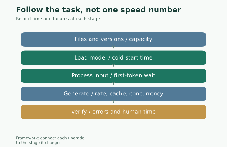
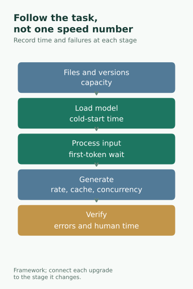
This division makes an upgrade claim testable. A faster SSD should be associated with a stage: acquisition, loading or generation. More memory should address an identified capacity constraint, while more bandwidth should address data movement. Without stage boundaries, two people can offer technically correct advice about different problems and appear to disagree.
2. Weight size is the beginning of the memory budget
A simplified starting point is weight bytes equal parameter count multiplied by bits per parameter, divided by eight. This ignores quantization scales, tensors retained at higher precision, indexing and runtime overhead. It is a baseline for understanding size, not a prediction of a particular download or the memory required to run it.
| Assumed parameter count | 16-bit weights | 8-bit weights | 4-bit weights |
|---|---|---|---|
| 8 billion | 16GB | 8GB | 4GB |
| 14 billion | 28GB | 14GB | 7GB |
| 32 billion | 64GB | 32GB | 16GB |
| 70 billion | 140GB | 70GB | 35GB |
All values are decimal GB and represent only the ideal weight payload. They are not GPU recommendations. A model’s size label may itself be approximate, so the actual parameter count and files should be checked when operating near a capacity boundary. Small errors in the budget become important when the plan assumes nearly every available byte can be allocated.
Running the model also requires KV cache, temporary tensors, framework allocations and room for the operating system and other applications. With a discrete GPU, CPU memory and graphics memory do not become a single equally fast pool merely because their capacities can be added on paper. Software that moves data between them brings the connection into the performance problem.
Consequently, the arithmetic “32 billion parameters at four bits is around 16GB” does not establish that any 16GB graphics card is suitable. The ideal weights already approach nominal capacity before cache and temporary space. Actual quantization formats differ. Check the exact model and backend, then measure allocation after loading and during representative long inputs rather than assuming that no headroom is needed.
Quantization also needs a quality test. A smaller file and an acceptable result are separate achievements. For interview cleanup, build examples containing names, product identifiers, dates and dense numbers, then check whether a lower-precision version changes those critical details. For coding, existing test outcomes say more than a few fluent-looking completions.
Mixture-of-experts models introduce another distinction. Parameters activated for a step affect computational work, but they usually cannot replace total weights in a storage estimate. The exact loading and offloading design matters. Choosing graphics memory from the smaller active-parameter label alone can make the budget wrong before context and concurrency are even considered.
The most useful question is therefore not how many parameters a device can advertise support for. It is which exact model configuration can complete your workload, with sufficient headroom, at acceptable quality and latency. Parameter count becomes one input to that investigation rather than its conclusion.
3. Context and concurrency can consume the remaining space
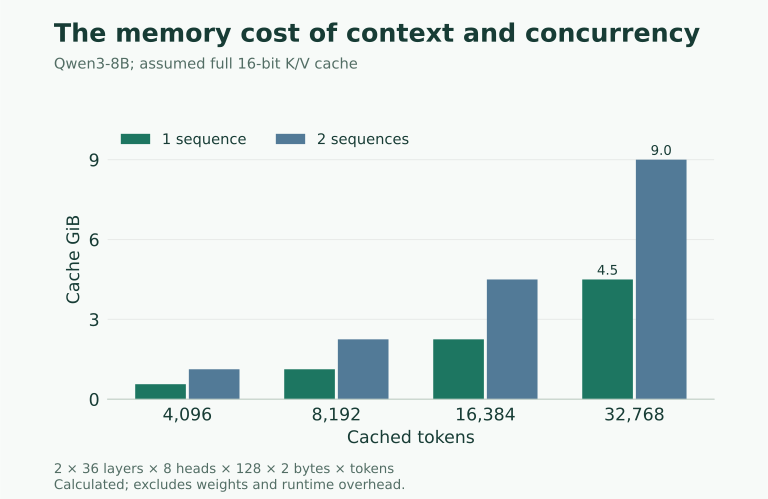
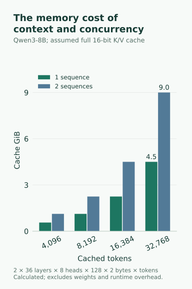
Long conversations preserve state for subsequent generation. A bounded example shows the scale. Qwen3-8B’s public configuration specifies 36 layers, eight KV heads and a head dimension of 128. Here we assume a conventional full-length, unquantized cache using two bytes per element, one sequence and no shared prefix. Qwen’s configuration.
The calculation is 2 for K and V × 36 layers × 8 KV heads × 128 dimensions × 2 bytes × tokens. That is 147,456 bytes, or 144KiB, per token. Context here means tokens stored, or capacity reserved for them by the framework. It is not a count of Chinese characters or English words.
| Cached tokens | Theoretical KV cache, one sequence | Two independent sequences |
|---|---|---|
| 4,096 | 0.5625GiB | 1.125GiB |
| 8,192 | 1.125GiB | 2.25GiB |
| 16,384 | 2.25GiB | 4.5GiB |
| 32,768 | 4.5GiB | 9GiB |
The calculation does not imply unlimited context support. Configuration, positional methods, implementation support and model accuracy on long material all constrain the useful range. Fitting the cache solves one resource problem; it does not establish that the model will retrieve an important fact reliably from a long document. That needs a separate task evaluation.
Framework behavior changes observed allocations. Some caches grow dynamically, some reserve space, and some support quantization or offloading. Hugging Face documents CPU/GPU movement for offloaded caches and latency trade-offs for quantized caches. Cache strategies. Memory savings can exchange capacity for other work rather than provide a free acceleration.
Ollama documents increasing memory needs with larger contexts and provides ollama ps to inspect placement. Its FAQ explains how parallel requests increase context-related allocation. Context documentation, concurrency documentation. These are version-sensitive behaviors: record the installed version and actual settings instead of copying a default from an old example.
In the interview workflow, one testable alternative is to check segments with a necessary terminology list rather than repeatedly insert the entire history. Segmentation can lose cross-segment information, so name consistency and merging require additional checks. If saving memory creates substantial human review, that work belongs in the budget rather than outside it.
Shared equipment also needs a queue policy. A successful single-session test does not promise the same latency for four simultaneous users. Test ordinary input, the longest commonly expected input and the intended concurrency. Otherwise the purchase has been validated only under the easiest conditions, while the difficult conditions remain an assumption.
4. Three product architectures address different constraints
The following comparison uses official specifications to show why capacity and bandwidth must be considered together. It is neither a recommendation ranking nor a current-price comparison. A complete system, an integrated platform and a discrete graphics card have different cost boundaries. Comparing a card’s purchase price with a whole computer without accounting for the host would be misleading.
| Representative configuration | Published capacity and bandwidth | The budgeting question it exposes |
|---|---|---|
| Mac Studio with M3 Ultra | 819GB/s; the support page checked lists 96GB base and a 256GB configuration | Unified memory is shared with the rest of the system; it cannot all be promised to one model |
| NVIDIA DGX Spark, 128GB configuration | 128GB unified system memory; 273GB/s | Relatively large capacity can coexist with lower nominal bandwidth |
| GeForce RTX 5090 | 32GB GDDR7; 1,792GB/s | High graphics-memory bandwidth can coexist with a tighter single-card capacity limit |
Sources: Apple specifications, DGX Spark specifications, and NVIDIA’s Blackwell white paper, page 15. These are manufacturer specifications, not tests for this article. Bandwidth across architectures cannot be converted directly into proportional tokens per second.
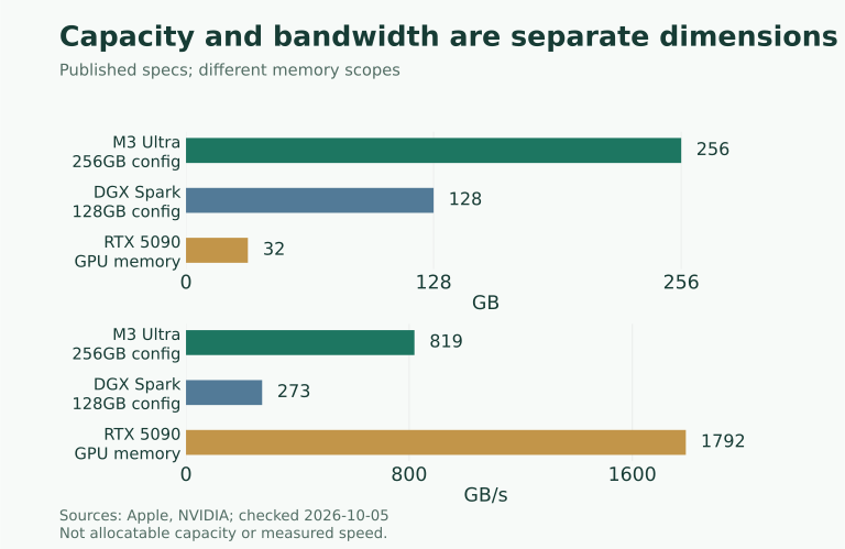
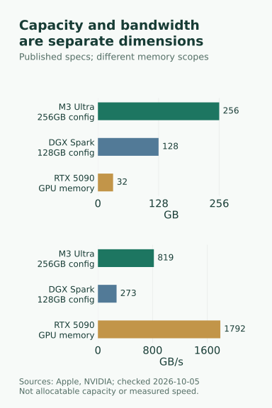
The industry insight is that manufacturers are serving different constraints. Some users need a larger model and working set on one machine. Others can fit a smaller configuration and prioritize throughput. Others chiefly need their existing software to work without major changes. Capacity, bandwidth, software support and integration are distinct capabilities that can each carry a price.
For the buyer, the question becomes which constraint binds first. If weights and cache cannot fit, headline bandwidth does not supply the missing space. If a model already remains resident, buying unused capacity may not improve generation. If the essential software lacks an appropriate backend, strong specifications may be unavailable to the intended workload.
Unified memory needs the same precision. It describes an access and organization approach, not a promise that the operating system consumes no space or every framework can allocate the full advertised total. Nor does it imply identical latency, bandwidth or optimization to dedicated graphics memory. Validate the backend, version, format and actual allocation.
Multi-GPU expansion should not be reduced to adding capacities. Model partitioning, communication, motherboard connections, power and cooling enter the result. Ollama’s description of cross-GPU loading itself discusses transfer considerations. Without a same-model workload test, two cards cannot simply be treated as one card with twice the capacity and twice the speed.
Specifications also have dates. Launch announcements, historical options and current support pages can differ, while regional offerings and inventory may differ again. The table uses explicit configurations visible at the time of checking; it does not survey local availability. Save the exact quoted configuration rather than buying from a remembered maximum.
5. Bandwidth supplies a bound, not a complete benchmark
For some single-sequence, autoregressive, dense-model decoding workloads, a deliberately simplified model is useful. If each generated token requires reading approximately W bytes of weights from the relevant memory level, and effective bandwidth is B bytes per second, that read alone gives a throughput ceiling around B/W. The purpose is to establish scale and expose assumptions, not predict a device’s measured output.
Suppose the weight traffic is 16GB per token and effective bandwidth is 100, 300 or 800GB/s. The simplified bounds are 6.25, 18.75 and 50 tokens per second. Those bandwidth values are hypothetical; they do not assign results to the devices above. Real execution also performs computation, reads cache, schedules kernels and handles quantization work, among other operations.
| Situation | What the simplified model omits | Additional measurement |
|---|---|---|
| First processing of long input | Parallel prompt computation and attention work | Time to first token and input throughput |
| Single-session generation | Cache traffic, effective bandwidth, kernels and compute | Steady output throughput and peak memory |
| Batched requests | Weight reuse, scheduling and queue time | Aggregate throughput and individual completion times |
| Experts or offloading | Active weights, routing and transfer paths | Stage timings and device-to-device movement |
This explains why a TOPS or FLOPS headline cannot by itself answer a local-user experience question. Peak compute depends on suitable precision, operations and utilization. A workload waiting for data may not benefit proportionally from more arithmetic capability. Another workload with intensive batched computation may value it greatly. The product number must be connected to the execution pattern.
Record prefill and decoding separately. Prefill processes existing input; decoding generates subsequent tokens. A model that waits three minutes and then writes quickly can have a similar average to one that starts after ten seconds but writes more slowly. Their usefulness in an interactive task can be very different. Time to the first useful result deserves its own place in the test.
Caching can also make a second run look unusually good. Comparing a loaded model with a reused prefix against a cold start on another machine changes state and hardware simultaneously. At minimum, distinguish cold start, a loaded model receiving a new request, and an intentionally reused prefix. Do not present the fastest condition as the experience available every day.
Keep the bound falsifiable. If a proposed explanation predicts that memory traffic dominates but measurement shows a long preprocessing step or CPU fallback, revise the explanation. A simple model helps only when its assumptions remain visible. Adding more decimal places to the same unsupported prediction does not make it a hardware test.
6. An SSD matters when its role in the task is identified
A larger SSD directly addresses insufficient file space. Faster reads may help frequent switching among large models. For a long-running model that remains resident, however, disk activity must be shown to affect the bottleneck before an SSD premium is credited with generation speed. Different stages can justify different purchases even in the same application.
Operating-system swap, framework weight offloading and KV-cache offloading are different mechanisms. Their data, triggers and access patterns differ. Summarizing them as software using disk, then describing an SSD as equally fast graphics memory, removes the decisive implementation and speed constraints. Whether an arrangement is acceptable is an end-to-end workload question.
A simple experiment is to fix model version, context and input and record the first load. Keep the model resident and submit a different request of similar length, recording generation separately. Then change the location of the model files and repeat the controlled conditions. If improvement belongs mainly to loading, describe it as a loading benefit rather than claiming that the model’s overall performance doubled.
External storage adds operational questions. Does the path mount reliably? Does it remain accessible after sleep? Can a background service read it? What happens when it is disconnected? Ollama’s OLLAMA_MODELS setting can select the model directory, but a changed path does not settle these conditions. Model-location documentation. One unexpected disconnect can undo the value of many slightly faster starts.
Keep the industrial pricing story separate as well. Data-center storage purchases do not map one-to-one onto a personal inference setup. They can change the importance of certain supply categories, while your capacity requirement still follows your files and workload. The companion article examines company data, price transmission and SSD budgeting.
7. A dock belongs in the whole connection path
Once a computer, dock, cable and SSD are connected, behavior is no longer a property of one product alone. Several fast-looking downstream ports do not imply that all devices can independently use the same uplink bandwidth at once. Check the host, upstream connection, downstream specifications and sharing arrangements.
| Connection element | Record before purchase | Check during acceptance |
|---|---|---|
| Host port | Exact computer and port protocol | Reported connection and direct baseline |
| Dock uplink and data ports | Upstream rate, downstream rates and sharing | One SSD alone versus additional active devices |
| Cable | Data capability separately from power rating | Whether a suitable alternative changes behavior |
| Displays | Resolution, refresh rate and independent-extension needs | Actual modes and stability for each display |
| Host power | Charger, dock host-output rating and cable conditions | Charging and connection stability under the real workload |
USB-IF distinguishes cable data capability from power markings, and the USB PD specification does not establish what every product delivers. Cable information, USB PD information. If an offer advertises 100W input, locate the actual host-output rating rather than assuming the figures are identical.
Display support is also model-specific. Apple’s guidance asks users to consider the Mac model, number of displays and operating modes. Apple display guidance. Two HDMI connectors do not establish that two independent extended displays will work. Driver-dependent arrangements introduce operating-system support, installation permission and maintenance questions.
A useful acceptance test can be straightforward: the same safe file set and SSD, first connected directly and then through the dock, with elapsed time and errors recorded. Add another shared device and observe the change. Replacing the cable, drive, files and operating system simultaneously makes attribution difficult, even if the final experience improves.
A dock can legitimately provide a tidier desk, easier connection and centralized ports. Those benefits should have their own budget rather than being confused with model performance. If direct connection already meets the speed requirement, paying for convenience can still be reasonable. The decision is clearer when the benefit is named accurately.
8. End-to-end cost can change the upgrade order
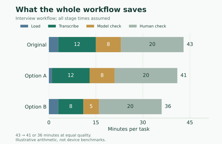
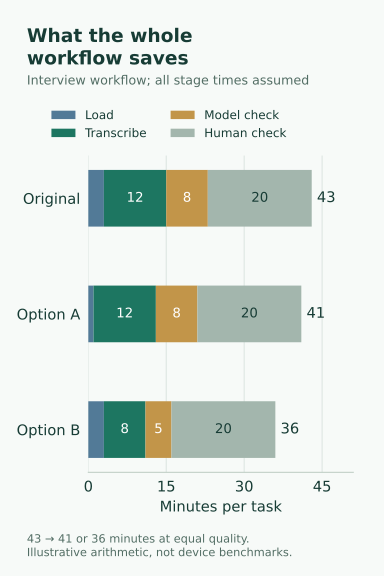
Return to the interview workflow and assume two entirely hypothetical alternatives. All outputs meet the same quality standard, and software fees are temporarily equal. The original process takes three minutes to load, twelve to transcribe, eight for text-model checking and twenty for human verification: forty-three minutes in total. Option A reduces loading to one minute, producing forty-one minutes overall. Option B reduces transcription to eight and text-model work to five, leaving the other stages unchanged: thirty-six minutes overall.
| Option | Total time per task | Time saved per task | Saving at an assumed 20 tasks per month |
|---|---|---|---|
| Original process | 43 minutes | — | — |
| A: faster loading only | 41 minutes | 2 minutes | 40 minutes |
| B: faster main compute stages | 36 minutes | 7 minutes | 140 minutes |
Large improvements to one stage remain bounded by the rest of the process. Human verification takes twenty minutes in all three scenarios. If a smaller, faster model adds ten minutes of checking, the apparent compute gain can be reversed. Keep the time record beside the quality standard instead of preserving only the best-looking performance measure.
Now add clearly hypothetical equipment premiums: RMB600 for A and RMB3,000 for B. At twenty tasks a month, annual savings are eight hours and twenty-eight hours. First-year equipment spending per hour saved is approximately RMB75 and RMB107 respectively. B is faster, but not cheaper on this particular measure. Neither number is a market quotation, and neither includes residual value, electricity or maintenance.
Double the workload and the result changes. Add another valuable use for the equipment and it should appear separately in the budget. If the purchase is for learning or enjoyment, the budget can reflect that purpose without claiming that every hour produces revenue. A specific account of use is more honest than applying a universal productivity percentage.
Cloud comparisons need an equally complete boundary. Include subscriptions or usage charges, transfer, availability, data-handling requirements and verification. A smaller local model and a stronger remote model are not automatically interchangeable units of output. Nor does local execution remove every data risk: permitted uploads, networked plugins and output storage still depend on the actual environment.
Organizations also incur deployment and maintenance work. Driver updates, framework compatibility, version rollback and fault handling may be done by the user or covered by a supplier. A more expensive arrangement that reliably supports essential software can provide integration value. Record the work it actually saves rather than assuming that every integrated product is economical.
Finally, distinguish elapsed time from occupied human time. A job that runs unattended overnight can be slow without blocking someone’s day, while a two-minute interruption repeated twenty times can be disruptive. The arithmetic above counts elapsed minutes. Turning them into economic value requires a separate judgment about how the workflow uses those minutes.
9. Three practical budget situations
An existing computer and modest text tasks. Begin with a small fixed test set, comparing model and quantization versions against quality and context needs. If the work completes reliably and storage is adequate, no hardware purchase is yet justified by the evidence. Improve prompts, document organization, verification and version records. A stable process creates the baseline needed to recognize a later hardware constraint.
Interviews, media and medium-sized local models. Record whether audio processing and text checking must remain resident together, then inspect peak memory and file growth. Serial execution may meet the deadline without buying permanent capacity for an occasional concurrent peak. If the deadline rules out serial work, the value of extra capacity has a concrete basis instead of being a general preference for larger specifications.
Long contexts, multiple sessions or large models. Define acceptable queueing, time to first token and output quality before comparing full tests on the relevant backend. The solution may involve unified memory, dedicated graphics memory, multiple GPUs or remote resources. Maximum parameter count is an incomplete ranking. Toolchain support, maintenance and a fallback when the setup fails become particularly important at this scale.
These situations provide an order of decisions rather than a fixed brand answer. Establish that software and model can perform the task, address the capacity or performance that limits it, and then decide what convenience is worth. When output is unreliable, upgrading does not replace validation. When the process is reliable, the next purchase should produce a measurable benefit.
10. Use an acceptance record to end endless specification comparisons
Before testing, fix the model identifier and file version, quantization, context, software, operating system and power mode. Prepare short, medium and long inputs that occur in real work, plus the expected concurrency. The aim is not a public benchmark leaderboard. It is a record that makes the difference before and after a purchase interpretable.
| Record | Minimum useful information | Misinterpretation it helps prevent |
|---|---|---|
| Identity and conditions | Model, backend, precision, context and configuration | Crediting hardware for a model or setting change |
| Cold start | Time from unloaded state to useful output | Presenting a resident-cache result as first-use behavior |
| Steady state | First token, generation rate and total time on new input | Hiding long-input waits behind output throughput |
| Resources | Peak memory, graphics memory, disk and concurrency | Validating only a small task or one user |
| Output quality | Errors and human correction under the same checklist | Trading quality for speed and calling it a net gain |
| Exceptions | Disconnects, failures, slowdowns and retries | Reporting only the successful run |
For an important workflow, repeat it enough to expose variation and describe that variation rather than retaining only the fastest value. Temperature, background activity and cache state can differ. Record conditions you cannot control. Silently dropping failed runs or moving retry time outside the total produces a less useful result even when the final number looks impressive.
Define an end to acceptance. The longest ordinary input completes, critical facts pass checking, repeated runs remain connected, and completion fits the work deadline: these are examples of usable criteria. Once they are satisfied, use the equipment. Without an end condition, a project intended to save time can become an indefinite comparison exercise.
The record also makes the next upgrade easier. If a model update becomes slower, check changed input length, cache settings, backend placement or task complexity. If hardware changes, retain the same workload baseline. This is much closer to the thing you are purchasing than restarting from a stranger’s description of something feeling smooth.
11. More hardware choices make workload discipline more valuable
Apple and NVIDIA specifications illustrate different paths through capacity, bandwidth and integration. They make more work possible on a desk while increasing the complexity of selection. An advantage on one axis cannot erase constraints on the others. That is why hardware variety makes a precise workload description more useful, not less.
Suppliers naturally display favorable measures. A buyer needs to translate them into task time, quality, operating limits and total expense. Every calculation in this article can accept different inputs. Disagree with the assumed frequency, model size or value of time, substitute your own figures, and the conclusion should be allowed to change.
Finish with a concrete purchasing requirement: this computer, this model version, this kind and length of material, this many simultaneous tasks, this deadline, this verification standard and this spending limit. Once that statement is clear, memory, graphics hardware, SSDs and docks each have an identifiable role. That makes the purchase explainable before money is spent and testable afterward.
Sources and method
Evidence checked October 5, 2026. No hardware benchmarks were conducted for this article, and no current prices or brand-performance ranking are offered. The weight table is ideal payload arithmetic. The cache example is bounded by the Qwen3-8B configuration and stated assumptions. Workflow times and premiums are hypothetical. GB is decimal; GiB is binary.
- Model and software: Qwen3-8B configuration, Hugging Face cache strategies, Ollama context, Ollama FAQ.
- Company specifications: Mac Studio 2025, DGX Spark, NVIDIA Blackwell white paper.
- Connections: USB-IF cables, USB PD, Mac displays.
- Reading time is estimated from the English prose at approximately 200 words per minute. Checking charts and calculations requires additional time.