# A 105GB model on a 32GB Mac: does a second SSD help?
Canonical: https://growthyoung.com/blog/moe-ssd-mirror-reads?lang=en
Author: Strategy Research Lab (Independent Research)
Published: 2026-10-07
Updated: 2026-10-07
Audit six mirrored-read runs, original outputs and file hashes. Separate throughput from waiting time, then use Qwen, Apple, Sandisk and OWC documentation to evaluate memory, storage and the software between them.
---
A Mac with 32GB of memory can run a model whose files occupy about 105GB. The useful explanation is in the software: it keeps frequently needed weights in memory and reads other weights when required. A second SSD can help only if the engine uses another read path. We checked a public six-run experiment, its output files and the relevant hardware specifications to work out what the evidence supports before turning it into an upgrade recommendation.
## 1. Where the model actually lives {#capacity}
Two questions keep coming up in discussions of local models. How can a computer generate an answer when the model files exceed its memory? And if an SSD participates in inference, can a larger or faster drive reduce the amount of memory someone needs to buy?
This article follows a community discussion about reading model weights from two drives into a public Slotstream experiment. Our audit means downloading the published records, checking file hashes, comparing six outputs and recalculating their measurements. We did not rerun the model on matching hardware. The machine and the original measurements belong to the experiment's author. The evidence cutoff is October 7, 2026.
A model file stores weights. During execution, the processor needs access to the relevant weights, while the program also keeps context state, temporary results and its own working data. Storage capacity accommodates the files. Working memory accommodates data in use. Software can move data between them, but that movement takes time and competes with other work.
A mixture-of-experts model, or MoE, makes selective movement possible. Each step activates a subset of expert networks. If some experts are used repeatedly, an engine can keep them in memory and leave others on disk. When a required expert is missing from the cache, its weights have to be read. How well this works depends on the access pattern as well as the cache policy.
The active parameter count therefore tells us about a different constraint from the size of the stored model. A small active subset can reduce the computation for one step while the whole collection of experts still needs a home. A later step can choose a different subset. Permanently deleting the currently inactive experts would change what remains available to the model.
Qwen's official model card describes Qwen3.8-Flash-Next as a 125B model with 6B active parameters, plus a 51B n-gram embedding and a 4B multi-token-prediction component. It lists 512 experts per layer, with 10 routed experts and one shared expert active. These are architectural quantities, rather than a measurement of this computer's memory use. [Qwen model card](https://huggingface.co/Qwen/Qwen3.8-Flash-Next).
| Number on the page | What it describes | What remains outside that number |
| --- | --- | --- |
| 125B parameters | Main model parameter scale | The separately listed n-gram embedding and MTP components |
| 6B active parameters | The active scale of one inference step | Inactive weights still need storage and may be selected later |
| About 105.3GB verified files | The pinned file set recorded for this experiment | Other versions and quantized repositories can contain different files |
| 32GB unified memory | The author's advertised machine configuration | The operating system, other apps, context and workspaces also need memory |
| 20.923GB peak footprint | The largest recorded process footprint in these six short runs | Longer inputs, concurrent requests and total system use |
The architecture values come from Qwen. The file set and machine description come from the author. We recalculated the final value from the six original statistics, using decimal GB. The machine record also distinguishes Apple's advertised capacity from the planner's decimal capacity accounting. [Machine and copy record](https://github.com/spikezz/slotstream/blob/mirror-reads/db/records/machines/mac-mini-m4-32gb.md).
A useful capacity exercise is 125 billion parameters multiplied by exactly four bits each. The result is 62.5GB of weight payload. That arithmetic excludes additional modules, quantization scales, metadata and tensors stored at another precision. A download larger than that estimate is entirely possible. A parameter label multiplied by one conversion factor is an incomplete purchasing budget.
Version identity matters too. Pipe Network's current quantized model card lists 103.8GB and explains the precision of different weight groups and the scope of its MTP files. The experiment records a verified set of about 105.3GB. We retain both definitions. The difference alone does not establish that a file is missing, and today's repository size should not replace the fixed set used in a historical experiment. [Quantized model documentation](https://huggingface.co/pipenetwork/Qwen3.8-Flash-Next-MLX-4bit).
## 2. A second drive needs a cooperating reader {#mirror}
Putting a model on an external SSD can immediately free internal storage. If the engine keeps reading only that directory, another idle drive on the desk will not accelerate it. The engine needs to know where another copy lives and actually schedule reads through it.
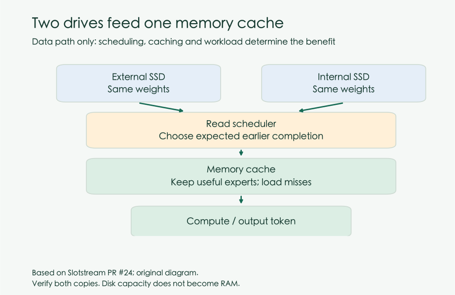
The proposed implementation is called mirror reads. Each physical drive stores an identical checkpoint. The reader uses observed throughput and queued work to select the copy expected to finish a request earlier. Replication gives a read request another destination. It adds storage use and another path for moving weights into memory. Its behavior differs from splitting the first half of the files onto one drive and the rest onto another. [Implementation and review status](https://github.com/carloslfu/slotstream/pull/24).
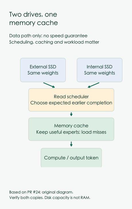
Figure 1. An original diagram of the documented data path. Arrows describe data movement, with no speed guarantee. A second drive does not automatically enlarge working memory.
| Arrangement | Where the data lives | Required support | Main cost or constraint |
| --- | --- | --- | --- |
| One model directory | One copy on one drive | An engine that reads the format | Capacity and performance of that path |
| Mirrored reads | Complete identical copies on two drives | Copy selection and concurrent reading in the engine | Duplicate capacity and copy verification |
| Split files | Different files on different drives | Support for the layout in the engine or storage layer | Hot files may concentrate work on one drive |
| Larger expert cache | More loaded experts remain in RAM | Available memory and a suitable cache policy | Less room for context, workspaces and other applications |
| Different quantization | A different representation of each weight | Support for the format and precision | Output quality needs a separate evaluation |
For replicated weights, correctness starts with the files. Matching filenames and lengths do not guarantee matching bytes. The author's record describes verification against a pinned file set on both copies. The PR also explains that startup checks of file sizes and headers cannot replace complete content verification. Switching between incompatible copies could produce faults that look like model or runtime problems.
Someone also has to maintain those two copies. A performance copy belongs under a fixed version manifest. A backup needs retention and restoration rules. Two model copies attached to the same working computer do not, by themselves, protect project files against accidental deletion, synchronized overwrites or loss of the whole machine. Decide what the additional drive is supposed to accomplish before budgeting for it.
## 3. What the six runs actually establish {#experiment}
The experiment uses a Mac mini M4 with 32GB of unified memory and macOS 15.7.4. The single-drive arm reads an external SSD. The mirror arm also uses an identical copy on the internal SSD. The machine record identifies a 2TB WD_BLACK SN8100 in an OWC Express 1M2 enclosure over Thunderbolt 4, alongside an approximately 251GB internal Apple SSD.
Both arms receive the same Chinese prompt, containing 47 prompt tokens, and generate exactly 200 output tokens. They use 118 cached experts per layer, an 8192-token context limit, MTP enabled and GPU keepalive disabled. Generation is greedy with a fixed seed. The order alternates: single then mirror, mirror then single, and single then mirror. The [protocol file](https://github.com/spikezz/slotstream/blob/mirror-reads/db/sources/artifacts/mirror-qualified-20261004/pairs/protocol.json) preserves the full settings.
| Pair and order | Arm | Generation, tokens/s | Generation, seconds | Prefill, seconds | Request, seconds |
| --- | --- | ---: | ---: | ---: | ---: |
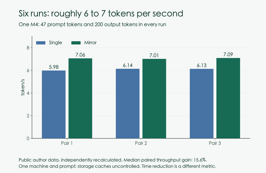
| Pair 1, first | Single | 5.983 | 33.425 | 10.459 | 43.966 |
| Pair 1, second | Mirror | 7.059 | 28.332 | 4.870 | 33.238 |
| Pair 2, first | Mirror | 7.012 | 28.524 | 4.878 | 33.437 |
| Pair 2, second | Single | 6.138 | 32.582 | 6.938 | 39.555 |
| Pair 3, first | Single | 6.132 | 32.618 | 6.930 | 39.584 |
| Pair 3, second | Mirror | 7.089 | 28.212 | 4.941 | 33.190 |
We checked the six original stats.json files against [rows.json](https://github.com/spikezz/slotstream/blob/mirror-reads/db/sources/artifacts/mirror-qualified-20261004/pairs/rows.json). Generation throughput is recalculated as 200 divided by decodeSeconds. Other times retain the recorded field definitions. In particular, requestSeconds excludes the separately listed load_seconds, so it should not be presented as the entire time from launching the program to finishing useful work.
We also downloaded all six output text files. Each SHA256 matches the published manifest. The output token arrays are identical across all runs, as are the prompt token arrays. The recorded global swap-in and swap-out counters do not increase between the before and after observations for any run. These checks establish consistency within the published evidence. They are not a rerun on independent hardware.
The measured source is identified as f37412f; the protocol provides the longer source and build identities. Later work rebased the PR and reorganized evidence. A reader reproducing the measurement should therefore distinguish the measured source from the latest commit displayed on the PR. At our cutoff the PR remained a draft. These results should not be described as a released feature already accepted by its maintainers.
## 4. A 15.6% throughput gain saves a different percentage of time {#metrics}
For each pair, divide mirror throughput by single-drive throughput and subtract one. The three improvements are 17.98%, 14.23% and 15.62%. Their median is 15.62%. If we instead divide the two arms' separately calculated median throughputs, the gain is 15.13%. Both calculations are well defined, but they summarize the measurements differently. A precise headline needs to say which one it uses.
Throughput and elapsed time also use different denominators. If speed rises from one to 1.1562, the time required for the same amount of work becomes approximately one divided by 1.1562. In these paired records, the median reduction in generation time is 13.51%. A person waiting for an answer experiences seconds. Choosing the larger percentage without explaining the metric creates an expectation the measurement never made.
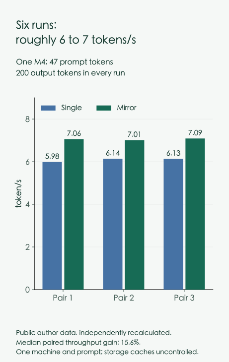
Figure 2. Original calculations and chart from the author's six records. Every run emits 200 tokens. The pairs share one machine and one prompt; they are not three independent hardware samples.
Separating the waiting stages is more useful. Prefill processes existing input. Generation produces subsequent tokens. Loading files, waiting in a queue and preparing state may add more time. A document-heavy task may spend much of its time before the first output; a short question followed by a long answer may spend more of its time generating. Average generation throughput describes only one part of that experience.
The median paired request-time reduction here is 16.15%, compared with 13.51% for generation alone. The difference follows from what each denominator includes. The first single-drive prefill took 10.459 seconds, while the next two were around 6.93 seconds. Prefill variability is visibly larger than generation variability in this small set. Keeping all six rows makes that visible.
The numbers do not assign a precise causal contribution to every subsystem. decodeIOSeconds is an engine counter. Prefetch can overlap computation, and instrumented intervals may contain one another. Adding that counter to total generation time would require checking whether it represents separate elapsed work. Subtracting it and calling the remainder pure GPU time would require similar evidence. We compare each field with its counterpart, without constructing an unsupported time budget from overlapping counters.
## 5. A fresh process does not clear every cache {#cache}
Each run starts a new process, rebuilding application caches. The experiment does not control the operating system's file cache or the SSD's internal state. The author records this limitation explicitly. It is a paired experiment under a fixed configuration, without a strict cold-storage guarantee.
That distinction changes how to interpret the first wait. Previously read files, earlier code execution and other machine activity can affect a subsequent run. The slower first single-drive prefill is worth investigating. Without measurements that isolate the cause, assigning that extra time to one particular cache would be speculation. A visible anomaly is a reason to preserve more evidence, rather than a license to invent an explanation.
Alternating AB and BA order helps because the same arm is not always first. It cannot make three pairs a large sample. Taking a median also does not erase the extra wait in the first pair. The original table remains useful precisely because it lets another reader judge the spread and decide what a follow-up experiment should control.
Context settings need the same care. An 8192-token configured limit does not mean the experiment actually processed an 8192-token input. It processed 47 prompt tokens. A long report with many rounds of tool output and images can change working memory, state retention and expert access. This record does not measure the latency of that workload, however large the configured limit looks on a screenshot.
A fixed 200-token output creates a compact comparison, but it does not establish completion of a user's task. Identical text supports the conclusion that the mirror arm did not gain speed by switching to a shorter or different answer. Whether that answer is correct, produces the requested tables or needs another round of prompting is a separate question.
For an agent that invokes tools, repeated failures belong in the timing record. Saving a few seconds on generation may contribute little if the agent repeatedly encounters the same tool error. Our [local AI upgrade budget](/blog/usb-c-hub-display-compatibility) discusses the cost of a completed task. The extra evidence here isolates part of the storage path so that it can be placed back inside the larger workflow.
## 6. Follow the connection before comparing drive specifications {#hardware}
The external drive's specification is an obvious source of excitement. Sandisk lists up to 14,900MB/s of sequential reading for the 2TB SN8100 and a PCIe Gen 5 x4 interface. That is a product capability under specified conditions. Once the drive sits inside an enclosure, data must also pass through its bridge, the cable, the host port and the filesystem. [SN8100 specifications](https://www.sandisk.com/en-ie/products/ssd/internal-ssd/wd-black-sn8100-ssd?sku=WDS200T1XHM-00CMT0).
Apple lists 120GB/s of unified-memory bandwidth for the 2024 M4 Mac mini. Its rear Thunderbolt 4 and USB4 connections support up to 40Gb/s, while the front USB-C ports support up to 10Gb/s. The uppercase and lowercase letters matter: 40 gigabits per second converts to a theoretical five gigabytes per second before protocol and other overheads. It is a separate path from the specified memory bandwidth. [Apple technical specifications](https://support.apple.com/en-au/121555).
| Company and measurement scope | Published number | Relationship to this experiment |
| --- | --- | --- |
| Apple, 2024 Mac mini specifications | M4 unified-memory bandwidth: 120GB/s | A memory-path specification, not external SSD speed |
| Apple, rear ports on the same model | Thunderbolt 4 and USB4: up to 40Gb/s | A host-side connection constraint; usable throughput is lower |
| Sandisk, SN8100 2TB specifications | Sequential reads up to 14,900MB/s; PCIe Gen 5 x4 | Drive capability requiring an appropriate connection |
| OWC, current Express 1M2 product page | Up to 3836MB/s on a specified Dell and OWC SSD combination | A vendor measurement on different equipment |
| Author's separate file-read experiment | QD4 medians: external 3.434GB/s, internal 2.223GB/s | A separately defined workload, not model token throughput |
OWC gives a test configuration in the footnote for its current number. Its 2023 launch material used a different platform for the advertised 3151MB/s figure. We treat those as results with different conditions; dividing one by the other would not measure an upgrade to the same system. [OWC product page and test footnote](https://www.owc.com/solutions/express-1m2).
The author also tested file reads at different queue depths and used device counters to check that disk reads occurred. We use its QD4 summary only to describe that experiment. Inference changes read sizes, dependencies and cache hits. Adding the internal and external GB/s values does not predict model tokens per second. [File-read summary](https://github.com/spikezz/slotstream/blob/mirror-reads/db/sources/artifacts/mirror-qualified-20261004/disk/summary.json).
A purchasing decision should follow the same physical route. Establish which drive holds the active model, which port it uses and which cable connects it. Only then ask whether another flash device or controller would address the measured constraint. A faster bare-drive specification may deliver little additional throughput through a slower connection. A matched experiment is still needed before declaring a particular drive either wasteful or necessary for the job.
## 7. A high cache-hit percentage can coexist with substantial reading
The recorded expertHitRate is approximately 80.9%. Read alone, that percentage might suggest storage is barely involved. Yet decodeReadBytes is around 23.5–23.6GB for only 200 output tokens. A relatively small fraction of misses can still move a substantial number of bytes. Hit counts and data volume describe different aspects of the workload.
A descriptive division gives about 0.118GB per output token from 23.6GB divided by 200. That is an average for this counter in this task. It is not a fixed requirement of all MoE models. It also describes reading, rather than writing that amount of data to flash for each token. Using a read counter as though it measured flash writes would create a false endurance argument.
Prefetch adds another layer. An engine can predict an expert needed soon and begin reading while it computes the current work. A useful prediction reduces waiting. An unused read still consumes resources along the storage path. The public statistics distinguish issuedBytes, adoptedBytes and wastedBytes. We do not add them to decodeReadBytes because their accounting scopes may overlap.
The value of a larger memory cache is that it can avoid some transfers entirely. But memory retained for experts must coexist with context, workspaces and other applications. A planner's expected peak for a full workload is also different from the observed peak in a short prompt. The approximately 20.9GB footprint here cannot guarantee that a nominally 32GB machine will have ample room during every longer session.
This gives software a direct role in the economics of an upgrade. The same SSD can produce different task throughput under another cache or prefetch policy. A software change can alter the marginal value of additional hardware. Keeping a baseline for the current version and workload is consequently more informative than shopping from an isolated hardware ranking.
## 8. Why doubling storage speed rarely doubles the whole task
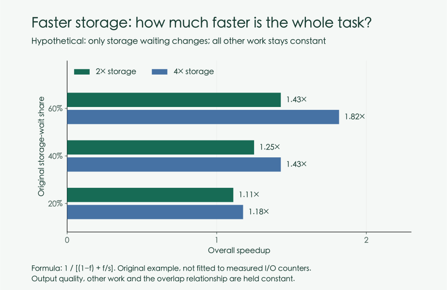
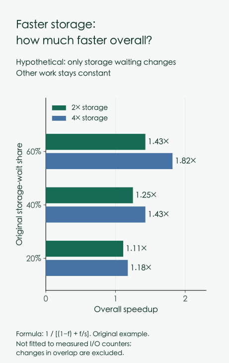
Consider an explicit hypothetical model. A fraction f of the original task time is unavoidable storage waiting. Other work remains unchanged. Speeding that storage portion up by a factor s makes the new time, relative to the old time, equal to (1−f)+f÷s. Overall speedup is the reciprocal. This is arithmetic for a serial decomposition, not a fit to Slotstream's overlapping instrumentation.
Figure 3. Original sensitivity calculations, not hardware measurements. Formula: 1÷[(1−f)+f÷s]. Other work, output quality and overlap are assumed unchanged.
| Original storage-wait share f | Overall speedup with 2× storage | Overall speedup with 4× storage | Limit if that wait disappeared |
| --- | ---: | ---: | ---: |
| 20% | 1.11× | 1.18× | 1.25× |
| 40% | 1.25× | 1.43× | 1.67× |
| 60% | 1.43× | 1.82× | 2.50× |
For f=40% and s=2, the task takes 80% of its original time. That is a 20% reduction in elapsed time and a speedup of 1.25. The example predicts no particular drive's performance. It makes a budget question explicit: if the affected stage occupies little of the task, even a very large improvement there has a limited effect on total waiting.
Real engines are less tidy. Prefetch can hide reads behind computation. Changes in queueing can affect other stages. A larger cache can change f itself. The formula helps frame measurements, but it cannot replace them. Dividing an I/O counter by total time and calling that ratio f would require evidence that the counter measures the serial waiting assumed by the model.
The same reasoning applies outside storage. Speeding up model generation leaves file conversion, tool execution and human checking untouched unless the workflow changes too. Readers can use this simple sensitivity calculation to ask which part of a proposed purchase actually affects their day, without pretending that a theoretical upper bound is a forecast.
## 9. Put the second drive inside a task budget {#budget}
The least expensive experiment often uses equipment already on hand. If there is enough internal capacity, an external model drive is already in use and the engine has a usable, verified mirror implementation, a fixed-task comparison can come before a purchase. The initial costs are occupied space, maintaining copies and the time needed to test them.
Buying another SSD and enclosure specifically for this feature requires a fuller budget. The following figures are invented planning assumptions, not current prices or observed savings. Suppose the incremental cost is RMB 900, there are 40 comparable requests per working day, each saves six seconds, and the month contains 22 working days. The calculation yields 88 minutes of machine waiting saved per month. If only one quarter becomes usable time, the result is 22 minutes.
That conversion depends on how someone works. A person watching for the first output may value a couple of seconds. Someone who starts a background batch and checks it in the evening may complete no additional work at all. Pricing every second of reduced machine time as saved labor overstates the benefit. A week of observing what changes in the actual routine can be more useful than assigning an optimistic hourly value.
| Situation | Evidence to inspect first | A reasonable next investment |
| --- | --- | --- |
| A small model already fits in memory and responds well | Whether generation still reads weights continuously | Preserve the baseline; another SSD may mainly add capacity |
| A large model waits on reads and two drives are available | Paired fixed-task time and output equality | Verify engine support, then test copy scheduling |
| Long reports produce slow first responses | Actual input length, prefill and reuse behavior | Check context and reuse policies before buying hardware |
| A tool-using assistant takes a long time without delivering | Tool failures, retries and usability of the result | Fix the failing stage and record completed-task time |
| A purchase depends on an unmerged feature | Release status, compatibility and fallback behavior | Wait for supported availability or accept experimental maintenance costs explicitly |
A smaller model is another candidate for the same task. It needs a separate comparison of answer quality and correction time, but a smaller parameter count is not enough reason to reject it. If the faster configuration repeatedly requires rewriting its output, the time saved during generation can disappear during review. The useful result is the object of the purchase.
Storage space has an opportunity cost as well. A full model copy competes with working documents, caches and recovery files on the internal drive. A performance improvement that forces constant manual cleanup can be a poor everyday arrangement. Record that maintenance in the budget instead of treating the second directory as free merely because the disk was already purchased.
## 10. What is worth tracking in the industry
The experiment suggests a specific purchasing relationship. Once software places weight reads on the inference path, storage performance can influence response time in more local-model workloads. The size of that influence depends on sparsity, caching, the connection and the task. A small experiment cannot establish a fixed increase in demand for every consumer SSD.
For chip and computer vendors, memory capacity and bandwidth continue to determine how much working data can stay available. For SSD and enclosure vendors, negotiated connections, sustained reading and latency stability become useful things to document. For engine developers, arranging reads under different memory budgets is a part of the system that software can improve. These are deductions from the data path; this article estimates no company's incremental revenue.
Product evaluation can follow that relationship. Alongside peak sequential reading, ask a report to identify the model revision, input length, expert cache, first and repeat waits, and output consistency. Those conditions connect component specifications to a user-visible outcome. They also help distinguish a gain due to hardware from one due to a changed engine or memory budget.
Our earlier [AI storage cycle article](/blog/portable-ssd-interface-capacity-workflow) examined supplier results and price transmission. This article examines reading within one workload. Each level needs its own evidence: an inference speedup cannot replace market-demand statistics, and a supplier's revenue growth cannot establish that a particular external drive should be upgraded.
For a buyer, the useful consequence is to preserve alternatives. Software improvements, a different model, a better connection or a larger memory budget may address different constraints. A benchmark that reports enough detail makes these choices comparable. A single headline number leaves them entangled, which makes it much harder to know what an additional purchase is supposed to fix.
## 11. How to repeat the comparison and change your mind {#verification}
Start with a task you actually need to complete. Preserve the input, model files, quantization, engine version and configuration. Mark capped or truncated output explicitly. Decide which measurements matter before running the comparison, so the final report does not silently choose whichever field happened to look best.
A practical starting design keeps the machine and task fixed and alternates single and mirror runs. Retain every result. Record engine request time as well as the time from startup to useful output, and inspect memory pressure and system swap. Repetition should reveal variability. Three pairs provide a limited clue; they cannot answer for every device and workload.
Separate first-use and repeated tasks. If operating-system and device caches are uncontrolled, label them that way. Do not replace the actual conditions with a loose claim of a cold start. Slow runs should remain in the record. If background activity interferes, preserve its circumstances and use a rule decided in advance to determine whether another complete comparison is required.
Correctness has several layers. File hashes check the input versions. Token IDs or output hashes check whether this comparison changed the answer. A real task still needs inspection of factual accuracy and successful tool actions. Passing one check does not establish the others. Two configurations can produce an identical wrong answer and therefore identical hashes.
The upgrade claim should be withdrawn if matched runs repeatedly produce different outputs, copies cannot be verified, the timing gain disappears in repeated comparisons, or the completed task does not become faster. A longer session that creates memory pressure should also prompt a new cache budget. Six short runs without swap cannot guarantee an entire afternoon under different conditions.
The conclusion from this audit stays narrow: on the author's single M4 machine, with a fixed short prompt, fixed output and manual settings, mirrored reads improved generation throughput in all three pairs. The median paired gain was about 15.6%. The published files are internally consistent under our checks. They do not promise the same gain on every Mac, MoE model or SSD. Before spending money, keep a baseline for your own task and let the additional equipment demonstrate what it saves.
## Data and calculation notes
AI assisted with source organization, calculations and editing. The underlying hardware experiment comes from a Slotstream contributor's public records. Our contribution is the file-consistency audit, recalculation, original figures and analysis; we did not independently run these hardware tests.
The records include the [measurement account](https://github.com/spikezz/slotstream/blob/mirror-reads/db/sources/runs/2026/10/2026-10-04-mirror-current-baseline-paired.md), [hash manifest](https://github.com/spikezz/slotstream/blob/mirror-reads/db/sources/artifacts/mirror-qualified-20261004/SHA256SUMS), [per-run data](https://github.com/spikezz/slotstream/blob/mirror-reads/db/sources/artifacts/mirror-qualified-20261004/pairs/rows.json), and each run's stats.json and stdout.txt. The retrieved rows.json had SHA256 `5e4b82d997a23db6f2d6e21b4dcb805a308b1a88043d56a61234ffe1b0eab928`. The source branch can change, so another audit should check versions first.
Tables round displayed values; percentages use the unrounded data. Byte calculations use decimal GB, while vendor capacities and bandwidth retain their published definitions. The sensitivity figure and the budget scenario are hypothetical and kept separate from measured results. This article has no product commission links and does not turn the six-run experiment into a purchasing ranking.
For your own calculations, download [our six-run data extract as CSV](/static/data/moe-mirror-read-audit.csv). It preserves the original field names, unrounded values and source dataset hash. The throughput column is calculated as 200 output tokens divided by generation time.